Electron Orbitals

Schrödinger Equation

Atomic Models

Bohr model

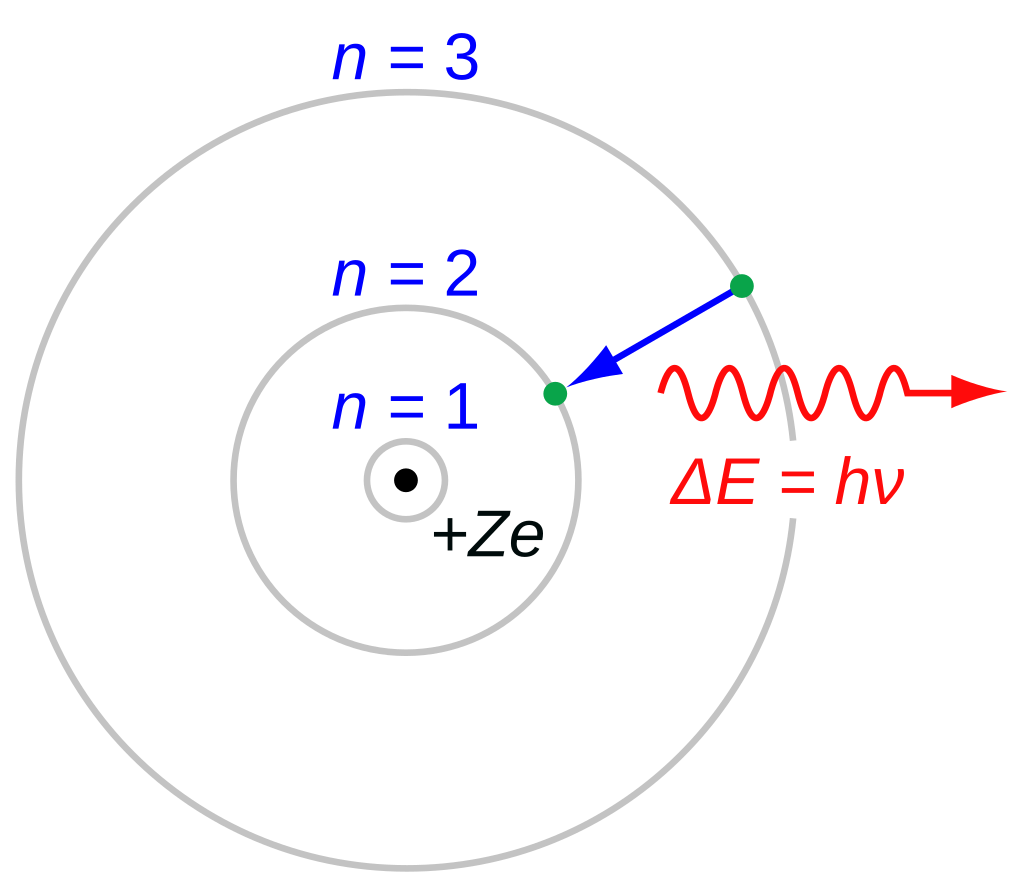
The Bohr model of the hydrogen atom (Z = 1) or a hydrogen-like ion (Z > 1), where the negatively charged electron confined to an atomic sh$\ell$ encircles a small, positively charged atomic nucleus and where an electron jumps between orbits, is accompanied by an emitted or absorbed amount of electromagnetic energy (hν). The orbits in which the electron may travel are shown as grey circles; their radius increases as _n_2, where n is the principal quantum number. The 3 → 2 transition depicted here produces the first line of the Balmer series, and for hydrogen (Z = 1) it results in a photon of wavelength 656 nm (red light).

Kvantová Čísla

Kvantové číslo je charakteristikou kvantového stavu.

Quantum Numbers

Schrödinger’s approach results in three quantum numbers that can be used to define an orbital (wave function), the principle ($n$), azimuthal ($l$), and magnetic ($m_l$) quantum number. There is a fourth quantum number, the spin quantum number ($m_s$) and electrons can reside in orbitals that are defined by these four quantum numbers. Every electron in an atom must reside in an orbital that contains a unique set of quantum numbers.^[1]

Principal quantum number ($n$)

Hlavní kvantové číslo^[2]

The principal quantum number (n) tells the average relative distance of an electron from the nucleus:

As n increases for a given atom, so does the average distance of an electron from the nucleus. A negatively charged electron that is, on average, closer to the positively charged nucleus is attracted to the nucleus more strongly than an electron that is farther out in space. This means that electrons with higher values of n are easier to remove from an atom. All wave functions that have the same value of n are said to constitute a principal shell because those electrons have similar average distances from the nucleus. As you will see, the principal quantum number n corresponds to the n used by Bohr to describe electron orbits and by Rydberg to describe atomic energy levels. As we will see, these can also be related to the periods of the periodic table.^[1:1]

Azimuthal Quantum Number ($\ell$)

Vedlejší kvantové číslo^[2:1]

The second quantum number is often called the azimuthal quantum number ($\ell$). The value of $\ell$ describes the shape of the region of space occupied by the electron. If you look at the standing waves in section 6.4.3.2 the value of $\ell$ can be related to the number of nodes and so the first standing wave ($n=1$) has $\ell =0$ (there is no node). The allowed values of $\ell$ depend on the value of $n$ and can range from 0 to $n-1$:^[1:2]

For example, if n = 1, $\ell$ can be only 0; if n = 2, $\ell$ can be 0 or 1; if n = 3, $\ell$ can be 0,1, or 2; and so forth. For a given atom, all wave functions that have the same values of both n and $\ell$ form a sub-shell. The regions of space occupied by electrons in the same sub-shell usually have the same shape, but they are oriented differently in space.^[1:3]

In naming orbitals we often denote the azimuthal number with a symbol. $\ell =0$ is an s orbital, $\ell =1$ is a p orbital, $\ell =2$ is a d orbital and $\ell =3$ is an f orbital. ^[1:4]

Magnetic Quantum Number ($m_{\ell }$)

Magnetické Kvantové číslo^[2:2]

The third quantum number is the magnetic quantum number ($m_{\ell }$). The value of $m_{\ell }$ describes the orientation of the region in space occupied by an electron with respect to an applied magnetic field.^[1:5]

The allowed values of $m_{\ell }$ depend on the value of $\ell$: $m_{\ell }$ can range from $-\ell$ to $\ell$ in integral steps:

For example, if $\ell =0$, $m_{\ell }$ can be only $0$; if $\ell =1$, $m_{\ell }$ can be $-1,0,\text{ or }+1$; and if $\ell =2$, $m_{\ell }$ can be $-2,-1,0,+1,\text{ or }+2$.

Each wavefunction with an allowed combination of $n$, $\ell$, and $m_{\ell }$ values describes an atomic orbital, a particular spatial distribution for an electron. For a given set of quantum numbers, each principal shell has a fixed number of subshells, and each subshell has a fixed number of orbitals.^[1:6]

Spin Quantum Number ($s$)

Spinové Kvantové Číslo^[2:3]

There is a fourth quantum number, which is the electron spin quantum number. The above three quantum numbers come from the solutions of the Schrödinger wave equation and describe the distance from the nucleus, the shape and orientation of the electronic orbitals that can exist for a hydrogen like atom. But there are actually two orbitals within each of these orbitals, and these result from the intrinsic spin of an electrons, which produces an intrinsic magnetic field. ^[3]

It should be noted that in 1928 Paul Dirac developed a relativistic wave equation, the Dirac Equation, that was consistent with both quantum mechanics and the theory of special relativity, and not only accounted for all four quantum numbers, but even introduced the concept of antimatter. ^[3:1]

Naming Orbitals

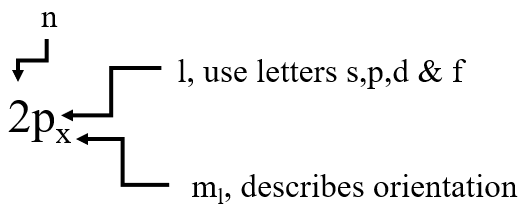
The first three quantum numbers define the geometric shapes of the orbitals and can be used to name them. The convention is to first indicate the principle quantum number (n), followed by a letter designating the azimuthal quantum number and then using a subscript to indicate the magnetic quantum number. The magnetic quantum number is often not specified. Note, the ml value may be the true values (-3,-2,-1,0,+1,+2,+3), or as we will see in the next section, expressions within the x,y,z Cartesian coordinate system.^[3:2]

Number of each orbital

For each shell there are n orbitals. The following table shows the allowed orbitals for ground state configurations, for each shell (principle quantum number) you add an azimuthal orbital (the allowed values of l for each n are 0 to n-1), where l=0 is an s orbital, l=1 is a p, l=2 is a d....)^[3:3]

As we shall see in the next Chapter, the structure of the periodic table is based on the filling of the orbitals in their lowest energy state, and the orbitals in orange (5g, 6g,6h,... are of such high energy that electrons do not occupy them if the electron is in a ground state configuration.^[3:4]

Now because the are $2\ell +1$ magnetic quantum numbers for each $n$, there are $n2$ potential orbitals for each principle quantum number.

n= 1 as one s orbital = (1 total)
n=2 has one s and three p (4 total)
n=3 has one s, three p and 5 d (9 total)
n=4 has one s, three p, 5 d and 7 f (16 total)

The Shape of Atomic Orbitals

In the previous section we learned that electrons have wave/particle duality, exist in orbitals that are defined by the Schrödinger wave equation that involves the complex coordinate system and imaginary numbers, and that they can be defined by quantum numbers n, l and ml. We use the Greek symbol psi ($\psi$) to represent a wave function. In this section we will look at the shapes of orbitals that have been transformed to the real coordinates of the x,y,z Cartesian coordinate system. The math of this transform is beyond the scope of this class, but for example, the $\psi P_{+1}$ and the $\psi P_{-1}$ orbitals can be combined in two ways that produce two new orbitals with real coordinates of the Cartesian coordinate system (the imaginary components of the wave functions cancel) the ${\psi }_{P_x}$ and ${\psi }_{P_y}$ orbitals. Since the original ${\psi }_{P_{+1}}$ and ${\psi }_{P_{-1}}$ were both solutions of the Schrödinger wave equation, their combinations are also solutions, and so we can visualize atomic orbitals as shapes along the x,y,z axes. All three quantum numbers influence the ultimate shape. The probability of finding an electron is ${\psi }^2$ and in the following representations we are implicitly defining the orbitals as the square of the wave-function.

So when we say $1s$ or $3d_{xz}$ we are orbital in terms of its location in space, and the images in Figure 6.6.1 represents the shapes of some common orbitals where there is roughly a 90% probability of finding the electron that resides in that orbital.^[4]

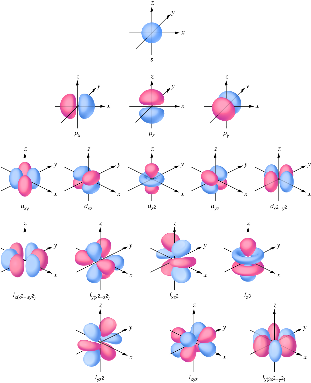
Figure 6.6.1: Select Cartesian coordinate visualizations of orbitals expressed in real space.

Note in Figure 6.6.1 that there is one type of s orbital $(l=0)$, three types of $p(l=1)$, 5 types of $d(l=2)$ and 7 types of $d(l=3)$. These are not the orbitals described the the magnetic quantum numbers, but combinations of them that result in the x,y,z Cartesian coordinate system.It should also be indicated that these represent the geometry for the first principle quantum number where an azimuthal quantum number occurs, so for example, this is the s orbital of the first shell, the p orbital of the second shell, d orbital of the third shell and the f orbital of the fourth shell.

s-orbitals

For l=0 the electron density function is spherically symmetric and the 1s orbital has no nodes. Figure 6.6.2 shows the square of the wavefunction.

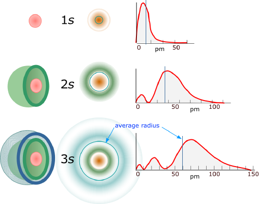
Figure 6.6.2: the radial distribution functions for the s orbitals of the first three principle quantum shells. This graph represents ${\psi }_{ns}^2$ for n=1,2 and 3 respectively.

As the principle quantum number ($n$) increases both radial nodes occur and the average distance from the nucleus increases. The "onion skin" analogy has often been used to describe this where the flesh of the onion represents the probability of an electron exisiting (realize the greater r, the greater the surface area), and the nodes are the empty spaces between the layers of the onion. Of interest is that the higher principle quantum number has the peak of its inner peak closer to the nucleus (the first peak in the ${\psi }_{3s}^2$ is at a shorter radius than for the ${\psi }_{2s}$ or ${\psi }_{1s}$.

p-orbitals

For the $n=2$ shell and greater there are three p orbitals. In the Cartesian coordinate the $p_z$ correlates to the $m_{\ell }=0$ and the $p_x$ and $p_y$ are mathematical combinations of the $m_{\ell }=+1\text{ and }{m}_{\ell }=-1$. (Note, the terms $p_x$, $p_y$ and $p_z$ actually relate to the wavefunctions squared, as indicated above.) For $n=2$ there is one node, in fact it is a nodal plane. If you look at the name, you can see that these are radially symmetric along one axis, which is the axis of the name, and the nodal plane is defined by the other two axes where they go through the origin. ^[4:1]

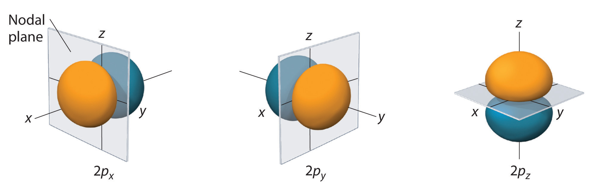
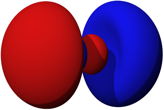
Figure 6.6.3: 2 p orbitals along the x, y and z axes (left) and a 3 p orbital (right).

Just as for s orbitals, as you move to higher principle quantum numbers the number of nodal surfaces increases, but they are no longer simple planar surfaces (see Figure 6.6.3). ^[4:2]

Practice